How Much Do Australians Know About Their Parliament?
It’s not often I see a cool data project focused on Australia, and in particular Australian politics, so I was especially excited to see freerangestats’ exploration of the 2016 Australian Election Study featured in RWeekly this week! The RWeekly email included this visualization, showing the responses to 6 questions about Australia’s parliamentary system, organized by party preference for Senate in the 2013 Federal Election.
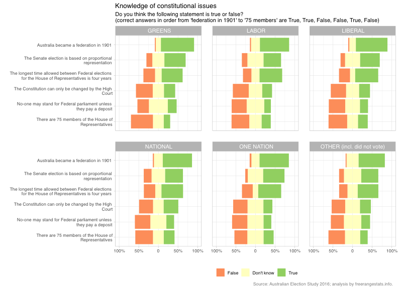
At first, I was excited to see where voters for my party came in relative to other voters in parliamentary trivia, but then… how can I even compare? I quickly realized that I have many qualms with this plot.
First, it takes some hunting to find the correct answers to each question (they’re listed in the subtitle), and once you’ve found them you have to go through six facets and match responses to answers. The plot shows the proportion of respondents who answered True, False or Don’t Know to each question. In my opinion, it would be far more intuitive to show only what we really care about: who was right!
Then there’s the choice of the stacked bar chart. Firstly, placing the “Don’t Know” responses at the middle, centered at 0, makes it almost impossible to see the percentages of “True” and “False” respondents, about whom we likely care far more. Secondly, the choice to make “False” go in the “negative” (labelled positive) direction on the axis, as well as the color choice, makes me intuitively assume that the orange indicates incorrect answers and green indicates correct.
Finally, what set me off in the first place: we can’t compare between parties! The orientation of the facets makes it very difficult to compare in the horizontal direction, even if the bars did all start at zero.
Here’s my proposed improvement on the visualization from freerangestats:
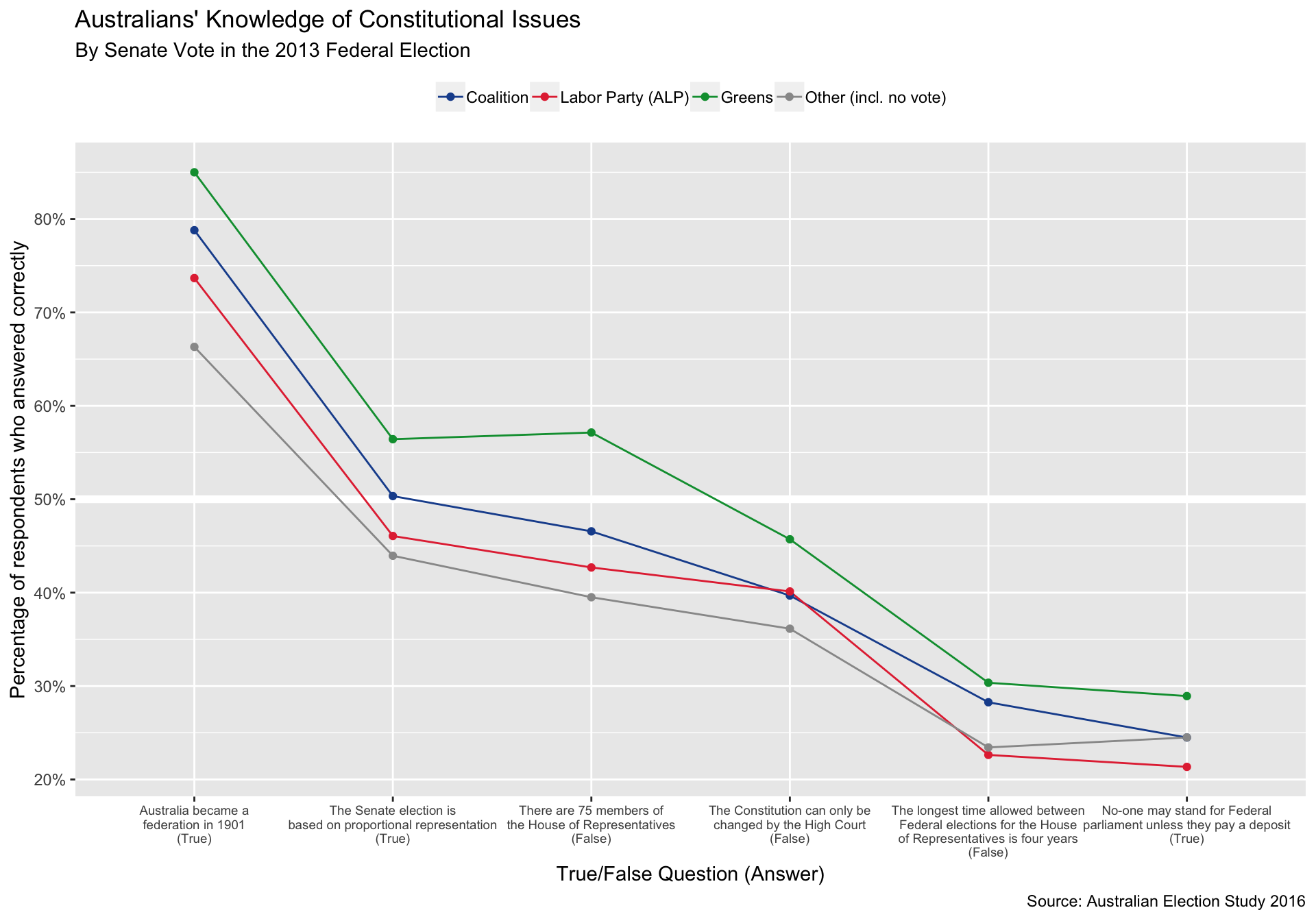
It looks from this plot like the Greens voters have outdone everyone across the board, followed by voters for the coalition. We shouldn’t draw any conclusions too quickly though, keep reading to see the code and explore how education levels influence Australian voters’ knowledge of their parliament.
Importing and Wrangling the Data
# Libraries
# =========
library(tidyverse)
library(haven)

# Constants
# =========
FILE_DATA <- "~/Data/aus-election-poll/aes2016.sas7bdat"
QUESTION_ABBRS <- c(
  "federation_1901",
  "prop_rep",
  "time_between_elections",
  "constitution",
  "deposit",
  "num_members_hrp"
)
QUESTION_LABELS <- c(
  "Australia became a\nfederation in 1901\n(True)",
  "The Senate election is\nbased on proportional representation\n(True)",
  "The longest time allowed between\nFederal elections for the House\nof Representatives is four years\n(False)",
  "The Constitution can only be\nchanged by the High Court\n(False)",
  "No-one may stand for Federal\nparliament unless they pay a deposit\n(True)",
  "There are 75 members of\nthe House of Representatives\n(False)"
)
QUESTION_LABELS_SHORT <- c(
  "Federation",
  "Proportional Representation",
  "Years Between Elections",
  "Changing the Constitution",
  "Deposit to Stand\nfor Federal Election",
  "Number of Members\nin the House of Reps"
)

PARTY_LEVELS <- c(
  "Coalition",
  "Labor Party (ALP)",
  "Greens",
  "Other (incl. no vote)"
)
PARTY_COLORS <- c("#1b4f9c", "#e43340", "#009c3d", "grey60")

EDUCATION_LEVELS <- c(
  "some secondary",
  "secondary",
  "trade",
  "university"
)
EDUCATION_LABELS <- c(
  "Some secondary school\nor less",
  "Secondary school only",
  "Trade Qualification\nor other Diploma",
  "Bachelor's Degree\nor higher"
)

# Functions
# =========
recode_truefalse <- function(x, answer) {
  recode(
    x,
    `1` = TRUE,
    `2` = FALSE,
    .default = NA
  ) %in% answer
}

recode_party <- function(x) {
  recode(
    x,
    `1` = "Coalition",
    `2` = "Labor Party (ALP)",
    `3` = "Coalition",
    `4` = "Greens",
    `997` = NA_character_,
    `998` = NA_character_,
    .default = "Other (incl. no vote)"
  )
}

recode_01 <- function(x) {
  if_else(x %in% 997:999, NA_real_, x)
}

import_vars <- list(
  weight = list(var = "wt_enrol", fun = identity),
  senate_vote = list(var = "B9_2", fun = recode_party),
  schooling = list(var = "G1", fun = recode_01),
  tertiary = list(var = "G3", fun = recode_01),
  federation_1901 = list(var = "F10_1", fun = function(.) recode_truefalse(., TRUE)),
  num_members_hrp = list(var = "F10_2", fun = function(.) recode_truefalse(., FALSE)),
  constitution = list(var = "F10_3", fun = function(.) recode_truefalse(., FALSE)),
  prop_rep = list(var = "F10_4", fun = function(.) recode_truefalse(., TRUE)),
  deposit = list(var = "F10_5", fun = function(.) recode_truefalse(., TRUE)),
  time_between_elections = list(var = "F10_6", fun = function(.) recode_truefalse(., FALSE))
)
The first step is to read in and wrangle the data. I downloaded the data in SAS format, so I use haven::read_sas to read the raw data. The list import_vars specifies the columns we would like to keep, the column names we would like to assign, and the functions we would like to apply to recode the survey response variables to a readable format.
There are many encodings in the survey data that should be recoded. For example, AES encodes “Item skipped” and “Does not apply”, responses we would like to encode as NA, as numbers 997 and 999. I also define functions to redefine the “True”/“False”/“Don’t Know” responses into logical vectors representing whether the respondent answered correctly, and to give names to the political parties. I chose to collapse the Liberal Party and the National (Country) Party into the Coalition, and drop One Nation to make the visualizations easier to digest.
I define my own education variable based on responses to two questions: “How old were you when you left secondary school?” and “Have you obtained a trade qualification, a degree or a diploma, or any other qualification since leaving school?”
df <-
  read_sas(data_file = FILE_DATA)

true_false <-
  import_vars %>%
  map_dfc(~ .$fun(pull(df, .$var))) %>%
  mutate(
    education =
      case_when(
        schooling > 1 ~ "some secondary",
        tertiary == 1 ~ "secondary",
        tertiary %in% c(2, 3) ~ "university",
        tertiary %in% c(4, 5, 6, 7) ~ "trade",
        TRUE ~ NA_character_
      ),
    education =
      factor(
        education,
        levels = EDUCATION_LEVELS,
        labels =  EDUCATION_LABELS,
        ordered = TRUE
      ),
    senate_vote = factor(senate_vote, levels = PARTY_LEVELS)
  ) %>%
  select(-schooling, -tertiary)
Visualizing Responses by Party
Now that the data has been cleaned up, I can create my version of the freerangestats visualization.
responses <-
  true_false %>%
  drop_na() %>%
  select(-weight, -education) %>%
  group_by(senate_vote) %>%
  summarise_all(mean, na.rm = TRUE) %>%
  gather(
    key = "question",
    value = "prop_correct",
    -senate_vote
  ) %>%
  mutate(
    question = factor(
      question,
      levels = QUESTION_ABBRS,
      labels = QUESTION_LABELS
    )
  )

responses %>%
  ggplot(
    aes(
      reorder(question, -prop_correct),
      prop_correct,
      color = senate_vote
    )
  ) +
  geom_hline(yintercept = 0.5, color = "white", size = 2) +
  geom_line(aes(group = senate_vote)) +
  geom_point() +
  scale_color_manual(
    breaks = PARTY_LEVELS,
    values = PARTY_COLORS
  ) +
  scale_y_continuous(
    breaks = seq(0, 1, by = 0.1),
    labels = scales::percent_format(accuracy = 1)
  ) +
  theme(
    axis.text.x = element_text(size = 7),
    legend.position = "top",
    legend.title = element_blank()
  ) +
  labs(
    title = "Australians' Knowledge of Constitutional Issues",
    subtitle = "By Senate Vote in the 2013 Federal Election",
    caption = "Source: Australian Election Study 2016",
    x = "True/False Question (Answer)",
    y = "Percentage of respondents who answered correctly"
  )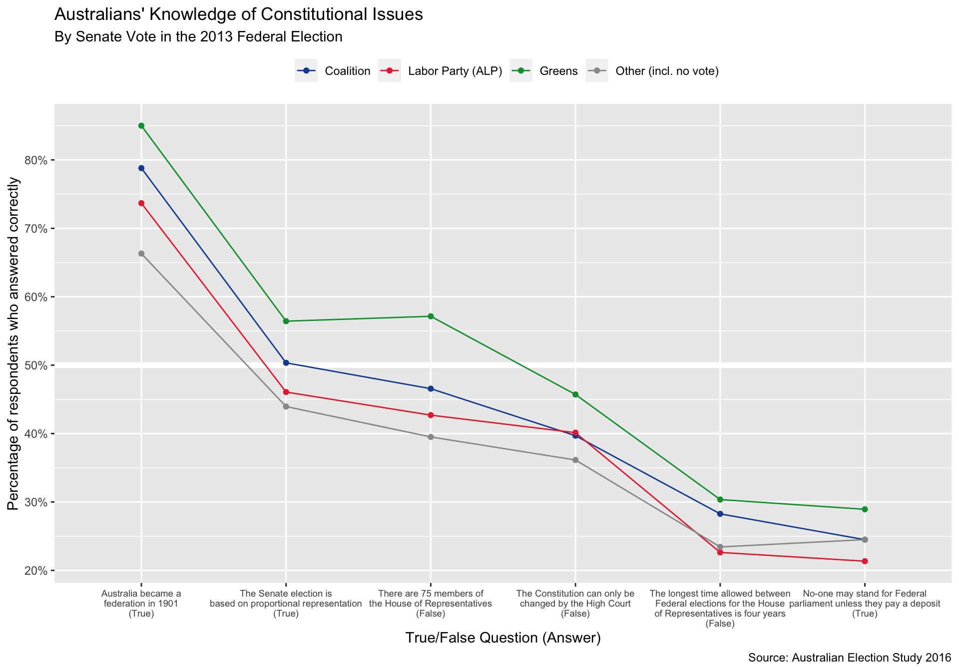
I think this plot is an improvement for a few reasons:
We can very easily compare between parties, and can very quickly identify parties by their official colors
We can quickly see the percentage of correct respondents
We can see which questions were easier and which were more difficult for the respondents
The answers are listed with the questions
There is some information lost, for example we can no longer see how many people said they didn’t know the answer, and it is much more difficult to figure out the raw responses. However, in my opinion this is far less important information in this context.
Controlling for Education Level
The AES gives us lots of details about the respondents including their education level. Although the plot above appears to indicate that Greens voters know the most about the parliamentary system, I was wary to jump to this conclusion without controlling for the level of education of the voters.
To make inferences about the enrolled population, we need to use the provided weights. Then we are able to calculate the proportion of the electorate and the proportion of voters for each of the Coalition, ALP and the Greens at each level of education.
total_ed_props <-
  true_false %>%
  drop_na() %>%
  count(education, wt = weight) %>%
  mutate(prop_educated = n / sum(n), group = "All respondents")

ed_props_by_party <-
  true_false %>%
  drop_na() %>%
  filter(senate_vote != "Other (incl. no vote)") %>%
  count(senate_vote, education, wt = weight) %>%
  group_by(senate_vote) %>%
  mutate(prop_educated = n / sum(n)) %>%
  ungroup()
Plotting these proportions shows dramatic disparities:
ed_props_by_party %>%
  ggplot(aes(education, prop_educated)) +
  geom_line(
    aes(group = group),
    color = "grey60",
    data = total_ed_props
  ) +
  geom_point(color = "grey60", data = total_ed_props) +
  geom_line(aes(group = senate_vote, color = senate_vote)) +
  geom_point(aes(color = senate_vote)) +
  scale_y_continuous(
    breaks = seq(0, 0.5, by = 0.1),
    labels = scales::percent_format(accuracy = 1)
  ) +
  scale_color_manual(
    breaks = PARTY_LEVELS,
    values = PARTY_COLORS
  ) +
  theme(
    legend.position = "top",
    axis.text.x = element_text(size = 8)
  ) +
  labs(
    title = "The highly educated are far overrepresented amongst Greens voters",
    subtitle = "Over 55% of Greens voters are university graduates, compared to 37% of the\n enrolled population (shown in grey)",
    x = NULL,
    y = "Percentage of voters by party\nweighted to match enrolled population",
    color = NULL,
    caption = "Source: Australian Election Study 2016"
  )
As we see in the plot above, university graduates are far overrepresented amongst Greens voters, while voters for Labor and the Coalition are reflective of national trends in education levels.
To understand whether educational differences account for the variation in performance on the True/False questions, we need to do some further exploration. To simplify this, I decided to calculate a score for each respondent. A simple and interpretable score is the proportion of correct answers to the 6 True/False questions.
scores <-
  true_false %>%
  drop_na() %>%
  mutate(
    frac_correct = (federation_1901 + prop_rep + time_between_elections +
                        constitution + deposit + num_members_hrp) / 6
  )
We can then visualize the distribution of scores at each education level.
scores %>%
  ggplot(aes(education, frac_correct)) +
  geom_hline(yintercept = 0.5, size = 2, color = "white") +
  geom_boxplot(varwidth = TRUE) +
  scale_y_continuous(labels = scales::percent_format(accuracy = 1)) +
  labs(
    x = "Highest Level of Education Attained",
    y = "Percentage of questions answered correctly (of 6 total)",
    title = "Median Performance Increases with Education Level",
    subtitle = "But performance varies widely at all levels",
    caption = "Source: Australian Election Study 2016"
  )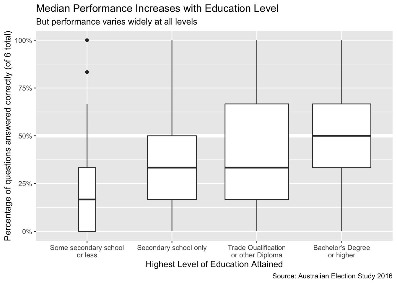
Despite the wide variation at every level of education, it does appear that university graduates performed the best on the multiple choice questions, with the top half of respondents with a Bachelor’s degree or higher getting at least half of the questions correct.
Finally, we can visualize the joint distribution of performance across the six questions, across the levels of education and across the party preferences. I chose to leave out those with less than a secondary school education, as this was a very small sample.
responses_with_ed <-
  true_false %>%
  drop_na() %>%
  select(-weight) %>%
  filter(education != "Some secondary school\nor less") %>%
  group_by(senate_vote, education) %>%
  summarise_all(mean, na.rm = TRUE) %>%
  gather(
    key = "question",
    value = "prop_correct",
    -senate_vote,
    -education
  ) %>%
  mutate(
    question = factor(
      question,
      levels = QUESTION_ABBRS,
      labels = QUESTION_LABELS_SHORT
    )
  )
responses_with_ed %>%
ggplot(
aes(
reorder(question, -prop_correct),
prop_correct,
color = senate_vote
)
) +
geom_hline(yintercept = 0.5, color = "white", size = 2) +
geom_line(aes(group = senate_vote)) +
geom_point() +
scale_color_manual(
breaks = PARTY_LEVELS,
values = PARTY_COLORS
) +
scale_y_continuous(
breaks = seq(0, 1, by = 0.1),
labels = scales::percent_format(accuracy = 1)
) +
theme(
axis.text.x = element_text(size = 9, angle = 45, hjust = 1),
legend.position = "top",
legend.title = element_blank()
) +
labs(
title = "Australians' Knowledge of Constitutional Issues by 2013 Senate Vote and Education Level",
subtitle = "University graduates outperform those less educated regardless of party affiliation",
caption = "Source: Australian Election Study 2016",
x = "Question Topic",
y = "Percentage of respondents who answered correctly"
) +
facet_grid(cols = vars(education))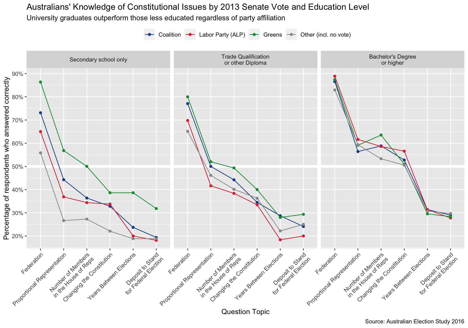
As we might’ve expected, the gap between voters across party preferences closes entirely with education level. Though it appears that accuracy amongst those with only a secondary school education does vary with party affiliation, this variation is much less pronounced amongst those with trade or other non-degree qualifications and completely indistinguishable amongst those with a university degree.
I will certainly be continuing to explore this data. I’m excited to think more about why the variation remains amongst secondary school graduates, or perhaps how socioeconomic status comes into play. It would also be interesting to break down the Coalition into Liberal voters and National Party voters. I’ll also be looking into some longitudinal analysis with the AES data!